
An Overview of AI Accelerators: MAC Operations, DRAM/SRAM, Performance Metrics, and Architecture
Learning from a classic AI accelerator - Eyeriss

I believe its important for people working around AI - ML engineers, semiconductor engineers, and end-users - to have a holistic understanding of AI, including the software interface and hardware underneath that optimizes calculations.
This primer focuses on AI accelerators: hardware designed to run deep learning efficiently. We’ll build intuition from the ground up (MACs → DNN/CNN structure → memory), explain the Von Neumann bottleneck, introduce the key performance metrics, and then ground everything in a classic example: Eyeriss.
This post synthesizes ideas primarily from “Efficient Processing of Deep Neural Networks” and “Eyeriss: An Energy-Efficient Reconfigurable Accelerator for Deep Convolutional Neural Networks.” Figures are adapted for educational commentary with attribution in captions; please see the original papers for full detail.
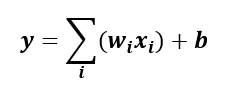
The compute: The Multiply- accumulate
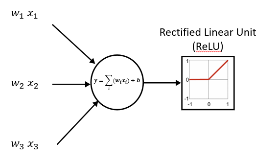
The Multiply - accumulation operation is the heart of most deep learning applications.
In simplest form,
then applies a nonlinearity (often ReLU). At the output, sigmoid (binary) or softmax (multi-class) can convert logits into probabilities.
There are few intuitions I use the thinking about Neural networks:
MAC operations are analogous to biological neurons: many inputs influence an output, and the weights determine what patterns the unit responds to. (It’s an analogy—not a literal model of the brain—but it’s a useful intuition.)
A neuron (dot product + nonlinearity) behaves like a pattern detector where the output is high in response to a input pattern that correlates with the combination of weights.
This multiple accumulate operation can be found across many range of deep learning applications.
Feedforward Neural Networks
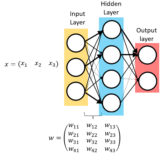
In feedforward neural networks, many of these neurons are assembled in parallel in a “pipelined” fashion. The inputs all connect to each “neuron”, each with its own unique set of weights to detect specific patterns, and these neurons then pass that information to later layers or the output. Additional layers can be added to be able to fine tune the pattern detection.
Adding “hidden” layers between the input and output allows the network to build up from simple features (edges/textures) to more complex features (higher-level shapes and objects).
There are two major operations performed on neural networks:
Training = learning the weights by passing images through, computing the error, and tuning the weights through “backpropagation”
Inference = running a trained model to produce outputs
Inference is commonly run on edge devices locally; training is usually done on large GPU/accelerator systems. Both training and inference can be run on GPUs or specialized accelerators optimized for these workloads.
Convolutional Neural networks
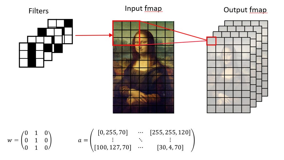
Convolutional neural networks (CNNs) are widely used for image recognition and classification. Instead of connecting every pixel to every neuron (which would explode parameter count and compute), CNNs use small filters that slide across the input in strides.
Each layer of the Convolutional Neural Networks operates in the following way:
Small filters represented as matrices can be customized to detect specific features, but the simplest case are “edge detectors” that detects vertical lines, horizontal lines, and diagonal dimensions.
These filters are “convolved” with each each input feature map (ifmaps), which is image pixel that is most commonly represented by a tensor of RGB values.
The output feature map (ofmaps) is calculated by sliding the filter across the input and accumulating partial sums (psums) along the way.
This feature map is condensed through normalization and “pooling” operations.
Each output feature map corresponds to a filter where the particular pattern is present (such as horizontal/vertical/diagonal line segments). As layers get deeper, higher order constructs are formed from simpler ones and spatial resolution shrinks. When dimensions are small enough, the CNN is connected to a fully connected layer that generates an output.
There are computational observations in both DNNs and CNNs as it relates to hardware:
Filter weights can be reused in computation without needing to retrieve it from memory every time.
The tensor shapes and data dependencies are known ahead of time, so you can pre-plan tiling and data movement to minimize expensive memory traffic.
These two points will become important later when we discuss Eyeriss.
The Von Neumann bottleneck
You have the best compute in the world, but it doesn’t matter if memory can’t keep up.
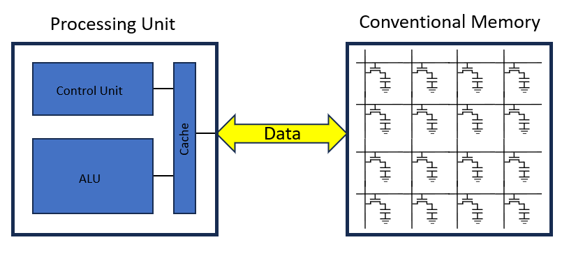
Most computing nowadays uses a Von Neumann architecture, where the compute and memory are split into two entities. Data stored in memory is retrieved and stored locally into CPU memory to perform operations on. When the result is computed, it is written back to the memory.
This architecture has worked as compute and memory are scaled. However, there are challenges being faced today:
Compute throughput has scaled faster than memory bandwidth/latency improvements
There is a limit transfer rate and a high energy cost per memory retrieval
This results in a bottleneck, where compute is limited by bandwidth + high energy per byte moved between memory and compute.
The question is, why don’t you put compute and memory on the same chip? You could, but its often not cost effective. Fab process for compute and memory optimize different things:
Logic (CPU/GPUs) are optimized for speed of transistor switching and ease of routing interconnects through stacking metal layers
Memory requires high density storage and capacity
One method classical computer architecture employs to mitigate this issue is arranging memory in a hierarchy through caches. Here, data is retrieved from the main memory only as “needed”. This exploits a phenomenon called “spatial locality” where you are likely to retrieve data close to the one you retrieved. As a result, you can write a whole data “chunk” of memory to a cache to increases the chances that you “hit” data in the cache when going to retrieve it.
AI Accelerators exploit both spatial locality and data reuse. In order to take advantage of both, we need to understand two mature memory technologies used across the hierarchy: DRAM, and SRAM.
The Memory: DRAM and SRAM
In a naïve implementation, each MAC operation requires three memory reads and one memory write:
Read: weight
Read: activation
Read: accumulated partial sum
Write: updated partial sum
To store data into memory, there are two mature memory technologies available:
DRAM - Dynamic Random access memory
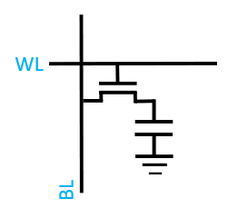
Figure 5. A DRAM cell with transistor and capacitor DRAM consists of capacitors that store charge and are read / written to word lines through a transistor. These memory cells are are typically arrayed in a 2D grid of cells with vertical row lines and horizontal bit lines. Memory cells are places at the intersection of word lines and bit lines where each ones is accessed by a combination of specific word line and bit line.
Pros: DRAM is cheap and dense.
Cons: DRAM is volatile and requires periodic refresh because capacitor charge leaks. It also requires constant electrical power to hold data.
SRAM - Static Random access memory

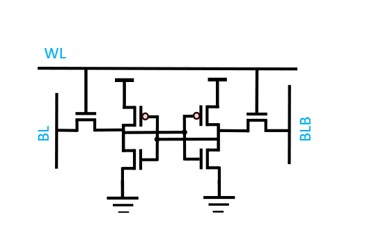
Figure 6. A 6 transistor SRAM cell with two inverters connected in a positive feedback configuration SRAM consists of cross coupled inverters in a latch (or positive feedback) configuration. The most common configuration is a 6 transistor cross coupled inverters to hold data. To read and store data, bitlines are charged and the wordline (WL) is activated depending on the values being read/written from/to the cell. The bitline needs to be strong (i.e. generate a lot of current) during write operations to break the feedback loop of the latches in order to flip the state of the memory cell. As with DRAM, these cells are arranged in a grid with these cells at the intersections.
Pros SRAM is faster and lower energy per access than DRAM. SRAM can also be easier to integrate on compute processes.
Cons: SRAM is much less dense and more expensive per bit.

Cost of memory: energy and bandwidth
There are two issues with DRAM:
The energy cost of DRAM is 1-2 orders of magnitude more expensive to access than on chip memory [1]. There are several factors that contribute to this, one of the largest being constant refresh cycles needed when non-ideal capacitors discharge through leakage paths.
The data bandwidth of DRAM is finite. In modern computer designs, DRAM is separate from the compute chips (CPU, GPU) and connected via busses with finite latency and throughput capabilities. In addition, DRAM itself has high latency due to steps of row activation, command delays, and precharging.
Due to the high energy cost, it is not desirable to read / write from DRAM continuously. Its better to read/write a “chunk” of information at a time and store the data locally on the chip to be accessed at memory technologies with lower energy cost.
There are a few trends that have been going on improve performance without significant changes to the Von-Neumann paradigm:
High bandwidth memory (HBM) - stacked DRAM integrated closely with the compute package to increase bandwidth.
Optimizing memory usage on chip into a memory “hierarchy”. When data is know in advance, it is possible to structure the data in a way that optimizes the memory cost and schedule data as such.
“Compute in/near memory” which uses more efficient memory technologies designed to handle this type of computation, or architectures design to do the computation by storing weights in conductance of resistors. There are many intriguing niche approaches here [2] but are beyond the scope of this post.
Performance metrics for DNN Models
“Performance” in a deep learning system consists of how performance is defined on both the model side and the Hardware side. Both are important and closely intertwined.
Metrics for DNN Models include:
Accuracy and robustness - How accurate is the model on common “benchmark” datasets
Network architecture - The number of layers, filters, and sizes
Number of weights - Affects storage requirements
Number of MAC operations
Often times, performance is compared in terms of normalized energy per MAC to give an apples to apples comparison of performance across different models.
Performance metrics for AI Accelerators
Hardware optimized for AI computation has its own set of performance metrics that that are optimized depending on the application:
Energy and Power is important for most applications, including cloud data centers with stringent power ceilings, as well as portable devices with limited battery
Low latency is important in real time interactive applications
High throughput is important for big data analytics is important when action needs to be taken based on the data
Hardware cost is important for most applications, when tightly integrating an AI chip on a consumer device to run inference, as well as integrating into a blade on a rack in a data center
Bridging Compute and Memory: Eyeriss [3]
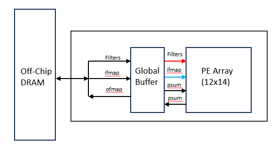
Eyeriss is a classic AI accelerator that optimizes for the deterministic nature of AI calculations. If you know the size and shapes of the filters, ifmaps, etc. you can optimize your flow to a given hardware set based on the size of the array. By doing so, you minimize the energy cost of moving data around.
Eyeriss has a few key building blocks:
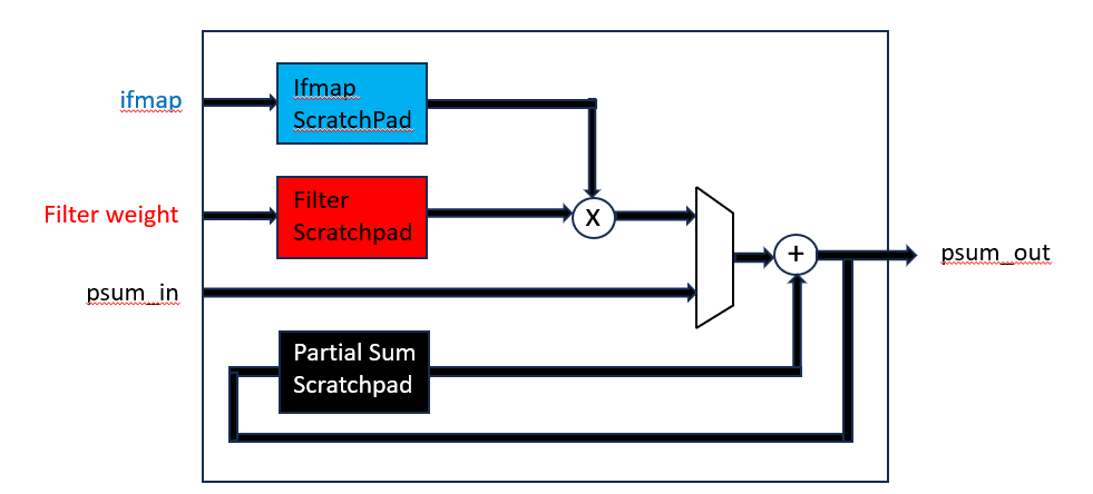
Processing Engine (PE)

Figure 8. Inside a Eyeriss Processing Unit. Adapted from Y.-H. Chen, T. Krishna, J. S. Emer, and V. Sze, “Eyeriss: An Energy-Efficient Reconfigurable Accelerator for Deep Convolutional Neural Networks,” IEEE Journal of Solid-State Circuits, early access, doi: 10.1109/JSSC.2016.2616357, 2016, Fig. 12; Figure is simplified and colored added for clarity. Each processing engine consists of a 16b two stage pipelined multiplier and adder, along with scratch pad memory to temporarily store the weights.
Data parallelism through Network on chip (NoC)
There are 168 processing elements arranged in a Spatial architecture of 12x14.
Each PE can communicate with neighboring PEs or the GLB through an NoC
The global input network handles the process of distributing the computations to each of the PEs though busses
Processing in each PE can be run independently from each other with data movement coordinated by the NoC
Four-level Memory Hierarchy
The memory hierarchy is arranged into four-level hierarchy in order of decreasing energy:
Off Chip DRAM
108kB global buffer
NoC reuse paths (neighbor PE communication)
Scratch pads local to PE (520 bytes each)
The goal of this chip is simple:
To minimize high cost DRAM and GLB access by reusing data from low cost spads and inter-PE communication as much as possible.
Eyeriss accomplishes this through a methodology called “Row stationary” that divides the matrix multiplication in a series of 1D convolution primitives that form 2D convolutional sets. :
1-D Convolution primitive in a PE
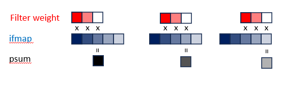
Figure 9. A 1D Convolution Primitive. Adapted from Y.-H. Chen, T. Krishna, J. S. Emer, and V. Sze, “Eyeriss: An Energy-Efficient Reconfigurable Accelerator for Deep Convolutional Neural Networks,” IEEE Journal of Solid-State Circuits, early access, doi: 10.1109/JSSC.2016.2616357, 2016, Fig. 3. Colors added for clarity A 1D convolution primitive can be best thought of as a “sliding window” approach because it ‘fixes” the filter weights in memory while the ifmaps are “slid” across it.
This allows weights/activations are reused many times before going back to DRAM and/or the GLB.
Accumulate psums from different primitives to generate the ofmap values

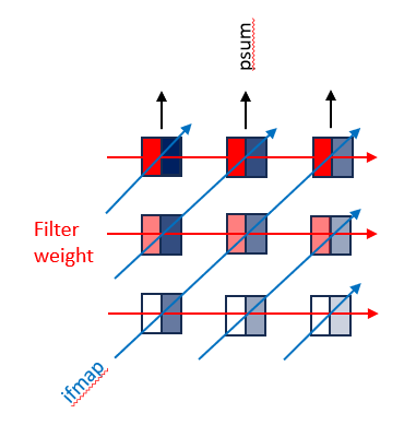
2D Convolution PE Set

Figure 10. A 2D Convolution Primitive with Constant value contours shown along the arrows. Adapted from Y.-H. Chen, T. Krishna, J. S. Emer, and V. Sze, “Eyeriss: An Energy-Efficient Reconfigurable Accelerator for Deep Convolutional Neural Networks,” IEEE Journal of Solid-State Circuits, early access, doi: 10.1109/JSSC.2016.2616357, 2016, Fig. 4; Colors added for clarity 2D convolution sets are formed from multiple 1D convolution primitives
In a 2D convolution set, the weight are written to spads in rows and the weights are “slid across” diagonally. It works in the following order:
Reuse each filter row horizontally
Reuse each of ifmap diagonally
Accumulate rows of psums vertically / features
The challenge is to “map” PE sets onto the PE array cleanly due to different sizes of layer shapes and PE array dimensions. Any computation primitive that exceed the size of the PE array itself or width / height can incur a large energy cost and needs further optimization from RS dataflow.
Other optimizations. These optimizations are also used and influential.
Run length compression - compress runs of 0’s
When distributing data from the GLB, only activate busses that correspond to the tag to save energy
A large fraction of the chip area goes to the memory, including the global buffer and on-chip storage close to the MACs.
Conclusion
In this primer I built up intuition of how AI accelerators optimize energy of AI computations:
MACs are the core primitive in most DNN workloads
DNN layers are repeated dot products with heavy weight/activation reuse potential
Performance is often limited by memory movement (energy + bandwidth), not arithmetic
Accelerators win by choosing dataflows + memory hierarchies that maximize reuse and minimize DRAM traffic
There is a lot of research done to optimizing AI accelerators including related compute near memory architecture that leverage traditional compute architectures as much as possible, as well as intriguing compute in memory approaches.
If you want to learn more about the technical developments of AI on the SW modelling side, check out my other post, based heavily on the book “Infinity Machine”:
From Atari to ChatGPT: The Technical and Corporate Forces Shaping Frontier AI

Demis Hassabis is perhaps one of the most important influences in Modern AI that isn’t a household name.
References
[1] V. Sze, Y.-H. Chen, T.-J. Yang, and J. Emer, “Efficient Processing of Deep Neural Networks: A Tutorial and Survey,” arXiv:1703.09039v2, 2017.
[2] A. A. Khan, J. P. C. de Lima, H. Farzaneh, and J. Castrillón, “The Landscape of Compute-near-memory and Compute-in-memory: A Research and Commercial Overview,” arXiv preprint arXiv:2401.14428, 2024.
[3] Y.-H. Chen, T. Krishna, J. S. Emer, and V. Sze, “Eyeriss: An Energy-Efficient Reconfigurable Accelerator for Deep Convolutional Neural Networks,” IEEE Journal of Solid-State Circuits, vol. 52, no. 1, pp. 127–138, Jan. 2017, doi: 10.1109/JSSC.2016.2616357.